this is the second part:
- OBIEE 12c Advanced Analytics Functions part 1. Introduction & Trendline
- OBIEE 12c Advanced Analytic part 2: BIN and WIDTH_BUCKET (this one)
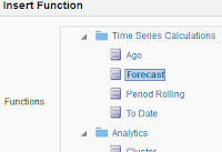
- OBIEE 12c Advanced Analytic part 3: Forecast
- OBIEE 12c Advanced Analytic part 4: Cluster
- OBIEE 12c Advanced Analytic part 5: Outlier
- OBIEE 12c Advanced Analytic part 6: Regression
- OBIEE 12c Advanced Analytic part 7: EVALUATE_SCRIPT
In this post I will talk about 2 functions with similar but somewhat different functionality: BIN and WIDTH_BUCKET.
Both functions aim is to define the bin / bucket the specific data entry belongs to. User can specify:
- Using what column the binning should be done- binned expression (it's a numeric expression / usually a measure).
- By what attributes it should be arranged; Please note the BY does not have the same meaning in both function.
- Number of Bins / Buckets and the type of data returned (one of 3: the bin / bucket number, it's min or max point).
- In Bin function there is also a where condition option for the BIN.
The major difference is the different meaning of the BY parameter and the fact that the BIN function result is treated as a Dimension Attribute while WIDTH_BUCKET is not.
The WIDTH_BUCKET itself is
one more "secret function", not available in the function menu.
For some reason, the syntax of the 2 functions is different.
More on the difference is available in the
documentation :
Note the following differences between the BIN and WIDTH_BUCKET functions:
- Unlike the BIN function, the WIDTH_BUCKET function is not treated as a new dimensional attribute for the purposes of aggregation. Instead, the WIDTH_BUCKET function is applied on top of the query result similar to the other display functions such as RANK, TOPN, BOTTOMN, NTILE, PERCENTILE, MAVG, and MEDIAN.
- The BY clause of the BIN function defines the grain at which the binned expression is evaluated prior to binning. If the binned expression is a measure, then the measure is grouped at the grain specified in the BY clause before being binned.
- The BY clause of the WIDTH_BUCKET function defines the groups in the query result set over which the WIDTH_BUCKET calculation is applied. The buckets within different groups are calculated independently.
- The BY clause of the BIN function is mandatory if the binned expression is a measure. Otherwise, for non-measure expressions, the BY clause is optional.
- The BY clause is always optional in the WIDTH_BUCKET function. If the BY clause is omitted from the WIDTH_BUCKET function, then the function operates over the entire result set.
- Use the BIN function when you want to compute a set of discrete buckets on top of a continuous valued attribute or measure and you want to treat that new set of discrete buckets as if it were a new dimension attribute that is intended to be included in the GROUP BY clause of other base measures in the query.
- Use the WIDTH_BUCKET function when you want to compute a discrete set of buckets on top of an already aggregated query result set.
Simple examples of both functions, then the syntax and few more examples.
Simple Example
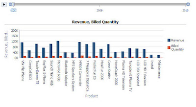
I'll use a "sample sales" based analysis With "Product Type", "Month" and "Revenue" columns.
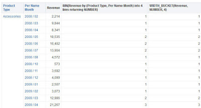
To place the Revenue values into 4 bins based on all the attributes of the analysis, I can get the same results with the following BIN and WIDTH_BUCKET function:
![]()
BIN:
BIN("Base Facts"."Revenue" BY "Products"."Product Type","Time"."Per Name Month" into 4 bins)WIDTH_BUCKET:
WIDTH_BUCKET("Base Facts"."Revenue", NUMBER, 4) ![]()
I had to define number of bins (4 in my case) in both functions (or get syntax error).
Few first differences:
The BIN function syntax is consistent with most Advanced Analytics in OBIEE while WIDTH_BUCKET is comma-based.
In BIN function I had to define the BY attributes (since "Revenue" is a measure) while I could omit them in WIDTH_BUCKET and accept the default.
Attempt to omit them in Bin function would cause an error in the Results Tab:
Error Codes: OPR4ONWY:U9IM8TAC:U9IM8TAC:U9IM8TAC:U9IM8TAC:OI2DL65P
State: HY000. Code: 10058. [NQODBC] [SQL_STATE: HY000] [nQSError: 10058] A general error has occurred. (HY000)
State: HY000. Code: 43113. [nQSError: 43113] Message returned from OBIS. (HY000)
State: HY000. Code: 43119. [nQSError: 43119] Query Failed: (HY000)
State: HY000. Code: 23058. [nQSError: 23058] The BIN expression requires a nonconstant BY clause if the expression being binned is a measure. (HY000)
The difference in meaning of BY
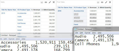
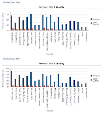
Now I will aggregate both functions BY "Month" and will show the different way each function interpretation of the meaning of it:
BIN:
BIN("Base Facts"."Revenue" BY "Time"."Per Name Month" into 4 bins)WIDTH_BUCKET:
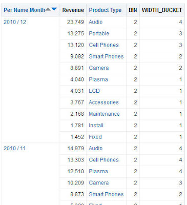
WIDTH_BUCKET("Base Facts"."Revenue", NUMBER, 4 by "Time"."Per Name Month") The result is not the same at all:
![]()
WHY?
The meaning of BY "Month" in WIDTH_BUCKET is: Take individual rows of data in each month and arrange them in 4 buckets.
The meaning of BY "Month" in BIN is: Take the sum("Revenue" by "Month") and arrange the sum of month in 4 bins. So rows of the same month will have the same BIN "Revenue" by "Month" results.
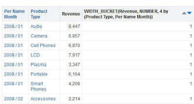
To be sure I understand it I asked myself, what would be the result of
WIDTH_BUCKET("Base Facts"."Revenue", NUMBER, 4 by "Products"."Product Type", "Time"."Per Name Month") Since all the data I have is combinations of the 2 attributes in the BY parameter, the function will return 1 for all the rows.
![]()
Returning
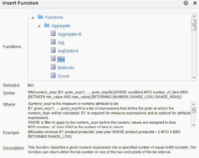
Before the formal syntax, what does the NUMBER parameter stands for in both functions?
It declares what the function should return. The Bin/Bucket number or the lower or the high value of the Bin/Bucket interval. The Possible values are: NUMBER, RANGE_LOW, RANGE_HIGH. we can have only one in each function. Here is the fist example with 3 WIDTH_BUCKET functions, each with a different Returning parameter:
![]()
And, naturally, the same result with BIN Function:
(For example, the BIN-High_Range formula is:
BIN("Base Facts"."Revenue" BY "Products"."Product Type","Time"."Per Name Month" into 4 bins Returning RANGE_HIGH) )
![]()
The Syntax of BIN:
BIN(numeric_expr [BY grain_expr1, ..., grain_exprN] [WHERE condition]
INTO number_of_bins BINS [BETWEEN min_value AND max_value]
[RETURNING { NUMBER | RANGE_LOW | RANGE_HIGH }])
Where:
numeric_expr indicates the measure or numeric attribute to bin.
BYgrain_expr1, ..., grain_exprN indicates a list of expressions that define the grain at which the
numeric_expr is calculated before the numeric values are assigned to bins. This clause is required for measure expressions and is optional for attribute expressions.
WHEREcondition indicates a filter condition to apply to the
numeric_expr before the numeric values are assigned to bins.
INTOnumber_of_bins indicates the number of bins to return.
BETWEENmin_valueANDmax_value indicates the minimum and maximum values used for the end points of the outermost bins.
RETURNING indicates a filter condition to apply to the
numeric_expr before the numeric values are assigned to bins. Note the following options:
RETURNING NUMBER indicates the return value should be the bin number (for example, 1, 2, 3, 4). This is the default condition.
RETURNING RANGE_LOW indicates the lower value of the bin interval.
RETURNING RANGE_HIGH indicates the higher value of the bin interval.
The Syntax of WIDTH_BUCKET:
The syntax of the WIDTH_BUCKET function is simpler than the BIN function, using simple comma-separated arguments instead of multiple clauses. The only nested clause supported by the WIDTH_BUCKET function is the BY clause, which is supported by all display functions including WIDTH_BUCKET, RANK, TOPN, and PERCENTILE.
WIDTH_BUCKET(numeric_expr, { NUMBER | RANGE_LOW | RANGE_HIGH },
number_of_bins, [min_value, max_value] [BY expr1, ..., exprN])
Where:
numeric_expr indicates the measure or numeric attribute to bin.
NUMBER indicated that the return value should be the bin number (for example, 1, 2, 3, 4). This is the default condition.
RANGE_LOW indicates the lower value of the bin interval.
RANGE_HIGH indicates the higher value of the bin interval.
number_of_bins indicates the number of bins to return. The default is 10.
min_value, max_value indicates the minimum and maximum values used for the end points of the outermost bins. If the
min_value and
max_value conditions are omitted, then the function determines the end points automatically
BYexpr1, ..., exprN indicates an optional list of expressions that define the groups in the query result set over which the WIDTH_BUCKET calculation is applied. The bucket intervals within different groups are calculated independently.
From the syntax we can see both functions have parameters (min_value, max_value) to exclude outermost points, if so desired.
One last BIN function examples:
The "where" example of BIN function:
I'll use the following function:
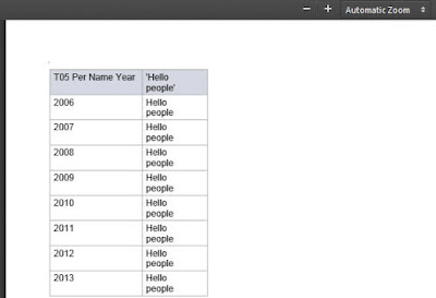
BIN("Base Facts"."Revenue" BY "Products"."Product Type","Time"."Per Name Month" where "Time"."Per Name Year"='2010' into 4 bins)Without any extra filtering.
![]()
The result is:
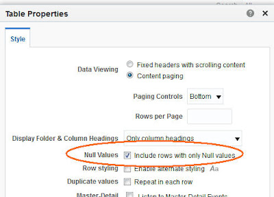
![]()
You can't see it in the picture, but as a result the data of the entire analysis is filtered to the Year 2010, since BIN has NULL values for any data that is not 2010. Turning on the "Include rows with Null values" option in the table properties would also return data with Null values in Revenue column.
![]()


 0
0